Example

Kelly (2007) provides a nice example of linmix in action. Here we reproduce these results.

First, we’ll import matplotlib for plotting, linmix, and numpy, and explicitly initialize the numpy random number generator for reproducibility:

import matplotlib.pyplot as plt
import numpy as np
import linmix
np.random.seed(2)

The example assumes the latent (unobserved) independent variable \(\xi\) is distributed as

\[\mathrm{Pr}(\xi) \propto e^\xi (1 + e^{2.75 \xi})^{-1}\]

We can simulate draws from this distribution using rejection sampling. First we plot the unnormalized density to find out what the maximum unnormalized probability is:

def pxi(xi):
    return np.exp(xi) * (1.0 + np.exp(2.75*xi))**(-1)
fig = plt.figure()
ax = fig.add_subplot(111)
x = np.arange(-5,5, 0.01)
ax.plot(x, pxi(x))
ax.set_xlabel(r"$\xi$")
ax.set_ylabel(r"$P(\xi)$")
plt.show()

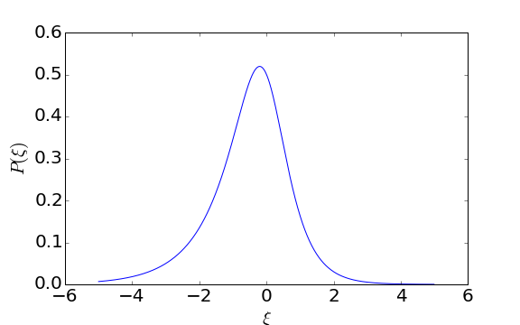
The maximum density is a little below 0.55, so we can use that. To draw samples from \(\mathrm{Pr}(\xi)\), we first propose a value \(\xi_i\) uniformly between -10 and +10 (it’s okay if we clip the tails for this example), and then keep that proposal if \(\mathrm{Pr}(\xi_i) > u\) where \(u\) is drawn uniformly between 0 and 0.55. If \(\mathrm{Pr}(\xi_i) < u\), then we propose a new value for \(\xi_i\). Here’s code to draw 100 samples from \(\mathrm{Pr}(\xi)\):

def rejection_sample(p, pmax, prop, size):
    out=[]
    for s in range(size):
        x = prop()
        px = p(x)
        pu = np.random.uniform(low=0.0, high=pmax)
        while px < pu:
            x = prop()
            px = p(x)
            pu = np.random.uniform(low=0.0, high=pmax)
        out.append(x)
    return np.array(out)
pmax = 0.55 # max p(xi) determined by eye
prop = lambda : np.random.uniform(low=-10, high=10) # truncating range to (-10, 10)
xi = rejection_sample(pxi, pmax, prop, size=100)

We can sanity check our samples by overplotting a histogram with the probability density function:

fig = plt.figure()
ax = fig.add_subplot(111)
x = np.arange(-5,5, 0.01)
ax.plot(x, pxi(x))
ax.hist(xi, 10, range=(-6,6), normed=True)
ax.set_xlabel(r"$\xi$")
ax.set_ylabel(r"$P(\xi)$")
plt.show()

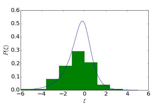
Looks reasonable. Now we set the regression parameters to see if we can reproduce them with the fit in a minute:

alpha = 1.0
beta = 0.5
sigsqr = 0.75**2
epsilon = np.random.normal(loc=0, scale=np.sqrt(sigsqr), size=len(xi))
eta = alpha + beta*xi + epsilon

Similarly, we initialize the (uncorrelated) 1-sigma error estimates, and using these, initialize the observed independent (\(y\)) and dependent (\(x\)) values. The observational errors are drawn from a scaled inverse \(\chi^2\) distribution as in Kelly (2007).

tau = np.std(xi)
sigma = np.sqrt(sigsqr)
t = 0.4 * tau
s = 0.5 * sigma
xsig = 5*t**2 / np.random.chisquare(5, size=len(xi))
ysig = 5*s**2 / np.random.chisquare(5, size=len(eta))
x = np.random.normal(loc=xi, scale=xsig)
y = np.random.normal(loc=eta, scale=ysig)

Let’s plot these to see what we got:

fig = plt.figure(figsize=(10,4))
ax = fig.add_subplot(121)
ax.scatter(xi, eta)
ax.set_xlabel(r'$\xi$')
ax.set_ylabel(r'$\eta$')
ax.set_xlim(-6,6)
ax.set_ylim(-3,4)
ax = fig.add_subplot(122)
ax.scatter(x, y, alpha=0.5)
ax.errorbar(x, y, xerr=xsig, yerr=ysig, ls=' ', alpha=0.5)
ax.set_xlabel(r'x')
ax.set_ylabel(r'y')
ax.set_xlim(-10,10)
ax.set_ylim(-5,6)
ax.plot([-6,6,6,-6,-6], [-3,-3,4,4,-3], color='k')
fig.tight_layout()
plt.show()

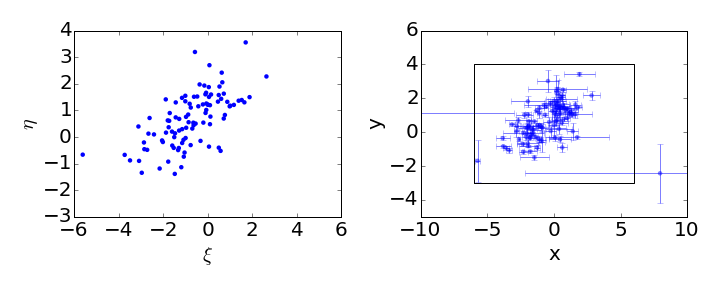
The left panel shows the distribution of the latent (unobserved) independent and dependent variables. The right panel shows the distribution, together with the error bars, of the observed variables. The rectangle on the right matches the figure outline on the left. The next step is to run the linmix algorithm on the simulated data

lm = linmix.LinMix(x, y, xsig, ysig, K=2)
lm.run_mcmc(silent=True)

We set K=2 here to use two components in the mixture model, which is reasonable for our fairly simple (and nearly Gaussian) latent independent variable distribution.

The code will run somewhere between 5000 and 100000 steps of a MCMC to produce samples from the posterior distribution of the model parameters, given the data. The code will automatically compare the variance of sample parameters between chains to the variance within single chains to determine if convergence has been reached and stop. If you want to see status updates as the code runs, then set silent=False or just leave the silent keyword out completely (its default is False).

When run_mcmc() has finished, we can see the output in the lm.chain attribute. Here we’ll plot the data and some samples from the Bayesian posterior on the same graph:

fig = plt.figure(figsize=(10,4))
ax = fig.add_subplot(121)
ax.scatter(xi, eta)
ax.set_xlabel(r'$\xi$')
ax.set_ylabel(r'$\eta$')
ax.set_xlim(-6,6)
ax.set_ylim(-3,4)
ax = fig.add_subplot(122)
ax.scatter(x, y, alpha=0.5)
ax.errorbar(x, y, xerr=xsig, yerr=ysig, ls=' ', alpha=0.5)
for i in range(0, len(lm.chain), 25):
    xs = np.arange(-10,11)
    ys = lm.chain[i]['alpha'] + xs * lm.chain[i]['beta']
    ax.plot(xs, ys, color='r', alpha=0.02)
ys = alpha + xs * beta
ax.plot(xs, ys, color='k')
ax.set_xlabel(r'x')
ax.set_ylabel(r'y')
ax.set_xlim(-10,10)
ax.set_ylim(-5,6)
ax.plot([-6,6,6,-6,-6], [-3,-3,4,4,-3], color='k')
fig.tight_layout()

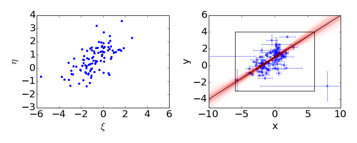
The black line shows the input regression line and the red lines show some samples from the posterior distribution.

Missing data

One of the advanced features of linmix is its ability to handle non-detections or missing data. For example, we can look at the case where we only consider a source detected if y>1.5. The delta array is used to indicate if a source is detected or not. In the code below, we feed the delta array into the LinMix constructor, generate MCMC samples the same way as before, and plot the results:

delta = y > 1.5
notdelta = np.logical_not(delta)
ycens = y.copy()
ycens[notdelta] = 1.5
lmcens  = linmix.LinMix(x, ycens, xsig, ysig, delta=delta, K=2)
lmcens.run_mcmc(silent=True)
fig = plt.figure(figsize=(10,4))
ax = fig.add_subplot(121)
ax.scatter(xi, eta)
ax.set_xlabel(r'$\xi$')
ax.set_ylabel(r'$\eta$')
ax.set_xlim(-6,6)
ax.set_ylim(-3,4)
ax = fig.add_subplot(122)
ax.errorbar(x[delta], ycens[delta], xsig[delta], ysig[delta], ls=' ', alpha=0.4)
ax.errorbar(x[notdelta], ycens[notdelta], yerr=0.3, uplims=np.ones(sum(notdelta), dtype=bool), ls=' ', c='b', alpha=0.4)
for i in range(0, len(lmcens.chain), 25):
    xs = np.arange(-10, 11)
    ys = lmcens.chain[i]['alpha'] + xs * lmcens.chain[i]['beta']
    ax.plot(xs, ys, color='g', alpha=0.02)
for i in range(0, len(lm.chain), 25):
    xs = np.arange(-10, 11)
    ys = lm.chain[i]['alpha'] + xs * lm.chain[i]['beta']
    ax.plot(xs, ys, color='r', alpha=0.02)
ys = alpha + xs * beta
ax.plot(xs, ys, color='k')
ax.set_xlabel(r'x')
ax.set_ylabel(r'y')
ax.set_xlim(-10,10)
ax.set_ylim(-5,6)
ax.plot([-6,6,6,-6,-6], [-3,-3,4,4,-3], color='k')
fig.tight_layout()
plt.savefig("cens_results.png")
plt.show()

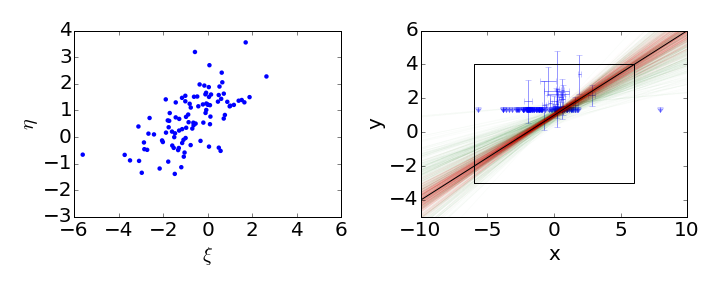
In this case, we use downward pointing arrows to indicate the upper limits on the non-detections. Again, the black line shows the input regression line, the red lines show samples from the posterior when no data is censored, and the green lines show samples from the posterior of the censored dataset. Linmix still does a good job of estimating the parameters of this challenging data set, in which only 21 of 100 points are detected.