linmix Math

Linmix is a hierarchical Bayesian model for fitting a straight line to data with errors in both the x and y directions. This model is described in detail by Kelly (2007) available here: http://arxiv.org/abs/0705.2774. The paper describes both univariate and multivariate models; since we have only implemented the univariate model to date, we only describe that model here.

The observed independent (\(x\)) and dependent (\(y\)) variables are assumed to be drawn from a 2-dimensional Gaussian distribution:

\[x, y \sim N_2(\mu, \Sigma)\]

with mean \(\mu = (\xi, \eta)\), which describe the unobserved true values the independent and dependent variables, and covariance matrix \(\Sigma = \left(\begin{smallmatrix} \sigma_x^2& \sigma_{xy} \\ \sigma_{xy} & \sigma_y^2 \end{smallmatrix}\right)\), where \(\sigma_x\) and \(\sigma_y\) are the \(x\) and \(y\) 1-sigma Gaussian errors and \(\sigma_{xy}\) is the covariance between \(x\) and \(y\).

The unobserved true independent and dependent variables are related by

\[\eta \sim N(\alpha + \beta \xi, \sigma^2)\]

where \(\alpha\) and \(\beta\) are the intercept and slope of the regression line and \(\sigma^2\) is the Gaussian intrinsic scatter of \(\eta\) around the regression line. The priors on the regression parameters \(\alpha\), \(\beta\), and \(\sigma^2\) are given as uniform.

The model for the distribution of the latent independent variable is a Gaussian mixture, which is both flexible and computationally manageable. The mixture is defined by the component probabilities \(\pi\), component means \(\mu\) and component variances \(\tau^2\):

\[\mathrm{Pr}\left(\xi|\pi, \mu, \tau^2\right) = \sum_{k=1}^K \frac{\pi_k}{\sqrt{2\pi\tau^2_k}}\exp\left[-\frac{1}{2}\frac{(\xi-\mu_k)^2}{\tau_k^2}\right]\]

The distribution of the mixture parameters \(\pi\), \(\mu\) and \(\tau^2\) are described by additional layers of the hierarchy:

\[ \begin{align}\begin{aligned}\pi \sim \mathrm{Dirichlet(1, ..., 1)}\\\mu \sim N(\mu_0, u^2)\\\mu_0 \sim U(\min(x), \max(x))\\u^2, \tau^2 \sim N(0, w^2)\\w^2 \sim U(0, \infty)\end{aligned}\end{align} \]

Note that we additionally truncate the domain of \(u^2\) to be \([0, 1.5 \mathrm{Var}(x)]\), as described in the notes of Brandon Kelly’s IDL program LINMIX_ERR.pro.

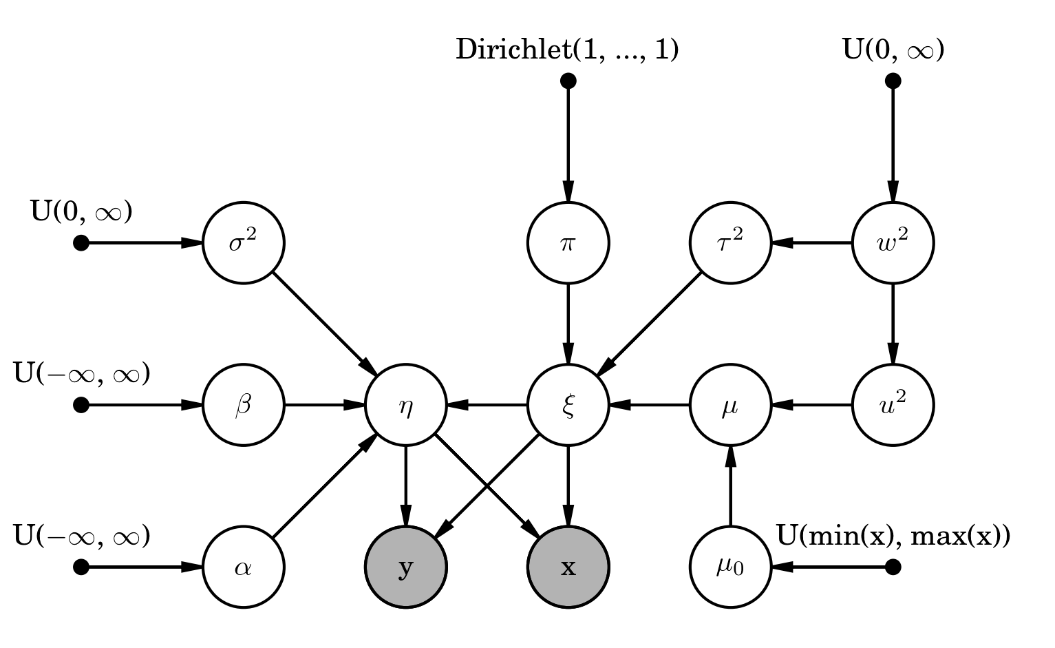
The entire model can be summarized by the following probabilistic graphical model: